45 how to add axis labels in excel 2013
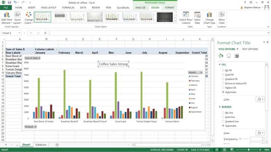
Adding rich data labels to charts in Excel 2013 | Microsoft 365 Blog To add a data label in a shape, select the data point of interest, then right-click it to pull up the context menu. Click Add Data Label, then click Add Data Callout . The result is that your data label will appear in a graphical callout. In this case, the category Thr for the particular data label is automatically added to the callout too. Excel tutorial: How to create a multi level axis To straighten out the labels, I need to restructure the data. First, I'll sort by region and then by activity. Next, I'll remove the extra, unneeded entries from the region column. The goal is to create an outline that reflects what you want to see in the axis labels. Now you can see we have a multi level category axis.
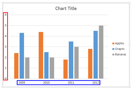
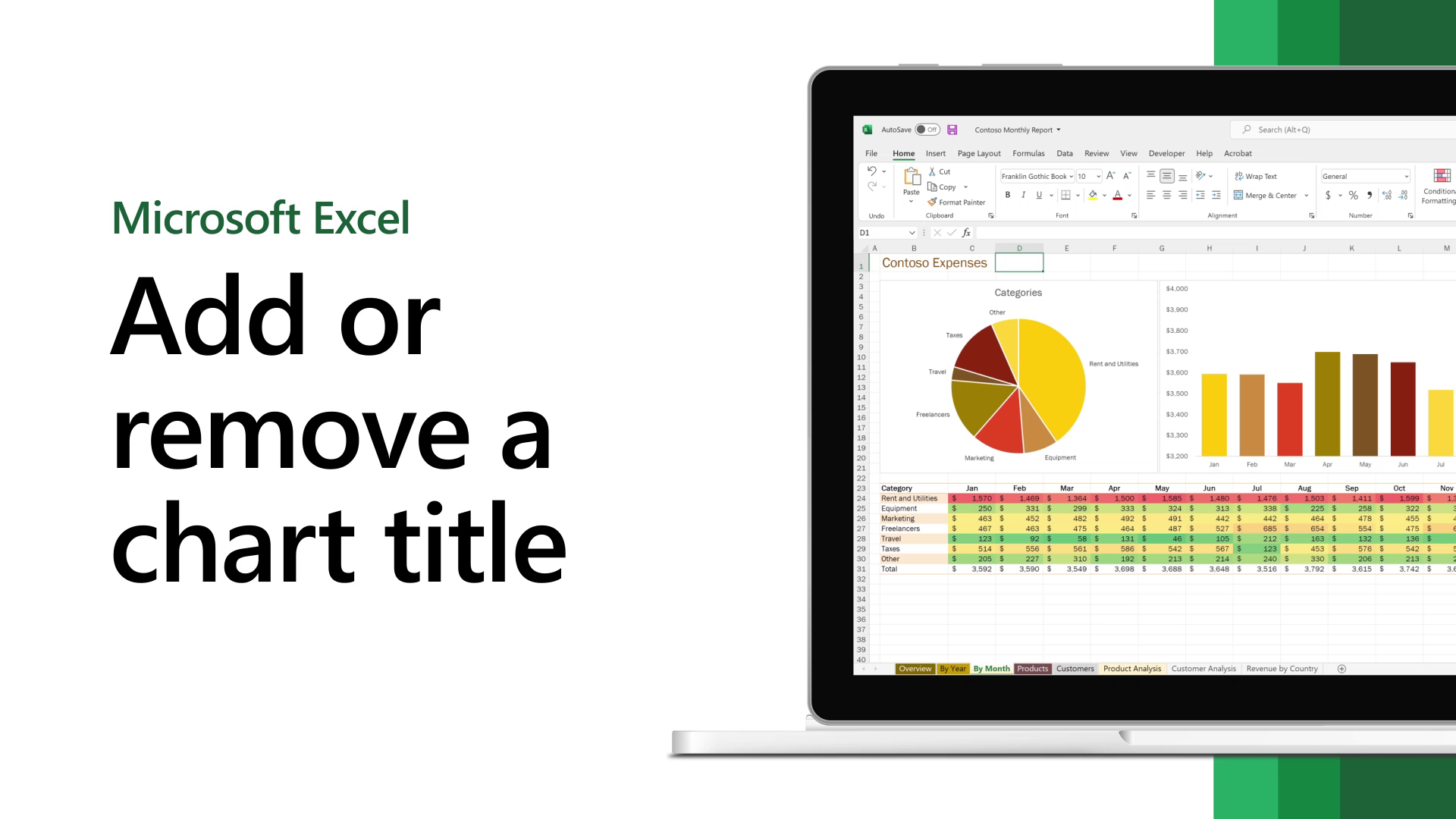
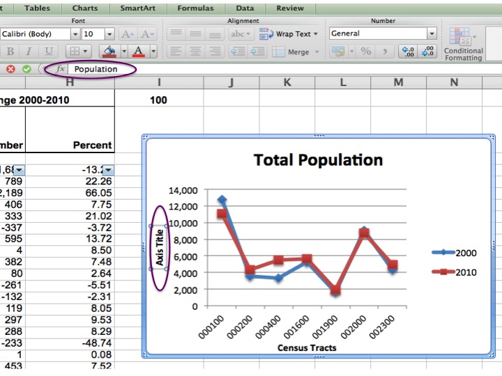
How to Add a Axis Title to an Existing Chart in Excel 2013 Watch this video to learn how to add an axis title to your chart in Excel 2013. A chart has at least 2 axis: the horizontal x-axis ...

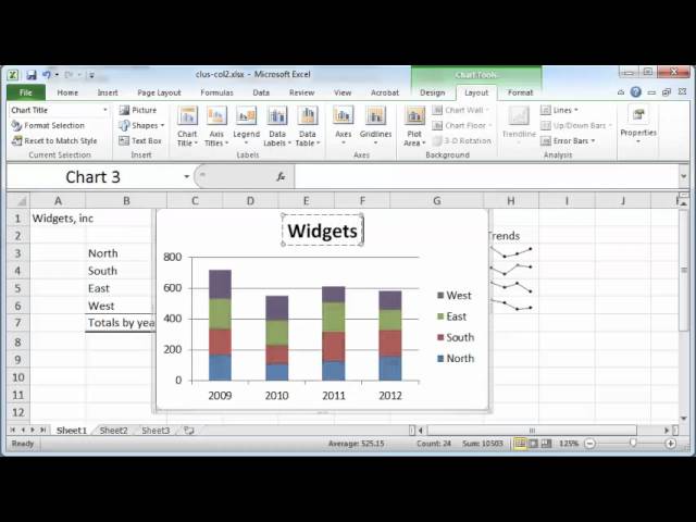
How to add axis labels in excel 2013
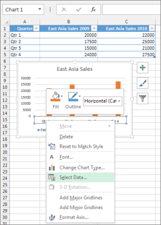
Two-Level Axis Labels (Microsoft Excel) - tips Put your second major group title into cell E1. In cells B2:G2 place your column labels. Select cells B1:D1 and click the Merge and Center tool. (In Excel 2007 the Merge and Center tool is in the Alignment group of the Home tab on the ribbon.) The first major group title should now be centered over the first group of column labels. Individually Formatted Category Axis Labels - Peltier Tech Format the category axis (horizontal axis) so it has no labels. Add data labels to the the dummy series. Use the Below position and Category Names option. Format the dummy series so it has no marker and no line. To format an individual label, you need to single click once to select the set of labels, then single click again to select the ... How to Create a Pareto Chart in Excel - Automate Excel Step #2: Add data labels. Start with adding data labels to the chart. Right-click on any of the columns and select "Add Data Labels." Customize the color, font, and size of the labels to help them stand out (Home > Font). Step #3: Add the axis titles. As icing on the cake, axis titles provide additional context to what the chart is all about.
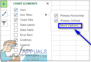
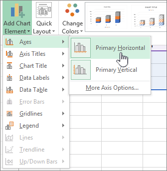
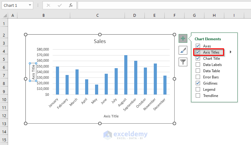
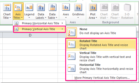
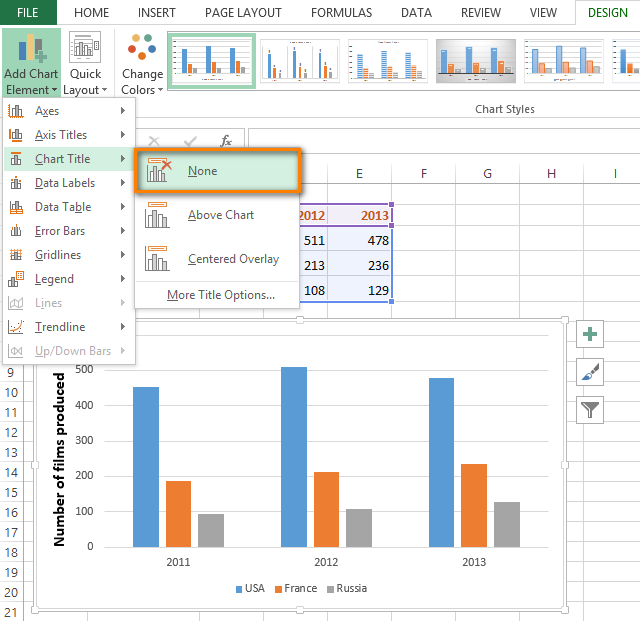
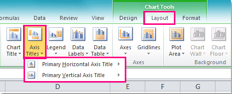
How to add axis labels in excel 2013. How to Add Axis Labels in Excel Charts - Step-by-Step (2022) - Spreadsheeto How to add axis titles 1. Left-click the Excel chart. 2. Click the plus button in the upper right corner of the chart. 3. Click Axis Titles to put a checkmark in the axis title checkbox. This will display axis titles. 4. Click the added axis title text box to write your axis label. How to rotate axis labels in chart in Excel? - ExtendOffice Rotate axis labels in chart of Excel 2013. If you are using Microsoft Excel 2013, you can rotate the axis labels with following steps: 1. Go to the chart and right click its axis labels you will rotate, and select the Format Axis from the context menu. 2. In the Format Axis pane in the right, click the Size & Properties button, click the Text ... How To Add Axis Labels In Excel - BSUPERIOR Go to the Design tab from the ribbon. Click on the Add Chart Element option from the Chart Layout group. Select the Axis Titles from the menu. Select the Primary Vertical to add labels to the vertical axis, and Select the Primary Horizontal to add labels to the horizontal axis. Picture 1- Add axis title by the Add Chart Element option How to add axis label to chart in Excel? - ExtendOffice In Excel 2013, you should do as this: 1. Click to select the chart that you want to insert axis label. 2. Then click the Charts Elements button located the upper-right corner of the chart. In the expanded menu, check Axis Titles option, see screenshot: 3.
How to Add Axis Labels in Excel 2013 - YouTube This is a tutorial on how to add axis labels in Excel 2013. Axis labels, for the most part, are added immediately to your chart once it is created. in Excel 2013, when the chart is highlighted, you... Custom Axis Labels and Gridlines in an Excel Chart In Excel 2013, click the "+" icon to the top right of the chart, click the right arrow next to Data Labels, and choose More Options…. Then in either case, choose the Label Contains option for X Values and the Label Position option for Below. The new labels are shaded gray to set them apart from the built-in axis labels. Excel: Labeling Sparklines - Excel Articles For the month labels below the chart, use a fixed-width font like Courier or Courier New. Type each month letter separated by a space. Make the font as small as possible. Center the values. Make the column width wider until the labels line up with the chart. Use the labels around the sparkline to add labels. Excel tutorial: How to customize axis labels Instead you'll need to open up the Select Data window. Here you'll see the horizontal axis labels listed on the right. Click the edit button to access the label range. It's not obvious, but you can type arbitrary labels separated with commas in this field. So I can just enter A through F. When I click OK, the chart is updated.
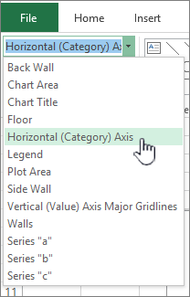
Excel Chart Vertical Axis Text Labels • My Online Training Hub To turn on the secondary vertical axis select the chart: Excel 2010: Chart Tools: Layout Tab > Axes > Secondary Vertical Axis > Show default axis. Excel 2013: Chart Tools: Design Tab > Add Chart Element > Axes > Secondary Vertical. Now your chart should look something like this with an axis on every side: How to Label Axes in Excel: 6 Steps (with Pictures) - wikiHow Open your Excel document. Double-click an Excel document that contains a graph. If you haven't yet created the document, open Excel and click Blank workbook, then create your graph before continuing. 2 Select the graph. Click your graph to select it. 3 Click +. It's to the right of the top-right corner of the graph. This will open a drop-down menu. Change axis labels in a chart - support.microsoft.com Right-click the category labels you want to change, and click Select Data. In the Horizontal (Category) Axis Labels box, click Edit. In the Axis label range box, enter the labels you want to use, separated by commas. For example, type Quarter 1,Quarter 2,Quarter 3,Quarter 4. Change the format of text and numbers in labels How to Add and Remove Chart Elements in Excel To add the data labels to the chart, click on the plus sign and click on the data labels. This will ad the data labels on the top of each point. If you want to show data labels on the left, right, center, below, etc. click on the arrow sign. It will open the options available for adding the data labels. 2: Add Vertical Gridlines to the Chart
How to Add Axis Titles in a Microsoft Excel Chart
Excel 2013: How to display corresponding text instead of numbers in ... Excel 2013: How to display corresponding text instead of numbers in axis labels? Ask Question. 0. I've a table of some task's progress, per person and I'd like to plot it on a chart. Y axis - names X axis - progress (NA, start, in progress, completed) and the preferable chart is bars, like that:

Microsoft Excel Tutorials: Format Axis Titles
How to group (two-level) axis labels in a chart in Excel? - ExtendOffice (1) In Excel 2007 and 2010, clicking the PivotTable > PivotChart in the Tables group on the Insert Tab; (2) In Excel 2013, clicking the Pivot Chart > Pivot Chart in the Charts group on the Insert tab. 2. In the opening dialog box, check the Existing worksheet option, and then select a cell in current worksheet, and click the OK button. 3.

Excel charts: add title, customize chart axis, legend and ...
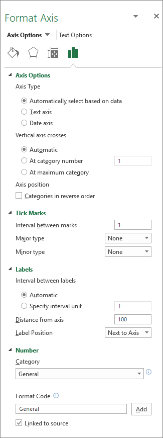
Changing Axis Labels in PowerPoint 2013 for Windows - Indezine Make sure you then deselect everything in the chart, and then carefully right-click on the value axis. Figure 2: Format Axis option selected for the value axis This step opens the Format Axis Task Pane, as shown in Figure 3, below. Make sure that the Axis Options button is selected as shown highlighted in red within Figure 3.
Microsoft Excel Tutorials: Format Axis Titles
How to Add a Secondary Axis in Excel Charts (Easy Guide) Below are the steps to add a secondary axis to a chart: Select the dataset. Click the Insert tab. In the Charts group, click the Recommended Charts option. This will open the Insert Chart dialog box. Scan the charts in the left pane and select the one that has a secondary axis. Click OK. Note: You also get other chart options that you can use.
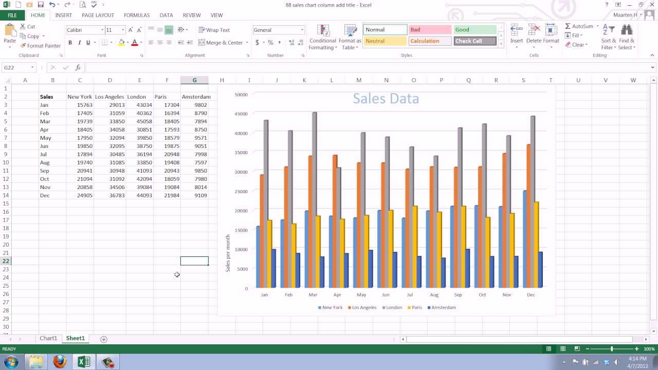
How to Add a Axis Title to an Existing Chart in Excel 2013
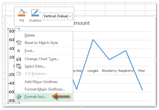
Adjusting the Angle of Axis Labels (Microsoft Excel) - ExcelTips (ribbon) Right-click the axis labels whose angle you want to adjust. Excel displays a Context menu. Click the Format Axis option. Excel displays the Format Axis task pane at the right side of the screen. Click the Text Options link in the task pane. Excel changes the tools that appear just below the link. Click the Textbox tool.

How to Add Axis Labels in Excel Charts - Step-by-Step (2022)
How to Add Secondary Axis in Excel (3 Useful Methods) - ExcelDemy Oct 03, 2022 · Eventually, this will open the Insert Chart dialog box. In the Insert Chart dialog box, choose the All Charts; Thirdly, choose the Combo option from the left menu. On the right side, we’ll find the data Series Names, 2 drop-down menus under the Chart Type heading, and 2 checkboxes under the Secondary Axis

How to Insert Axis Labels In An Excel Chart | Excelchat
How to Change Excel Chart Data Labels to Custom Values? May 05, 2010 · Col A is x axis labels (hard coded, no spaces in strings, text format), with null cells in between. The labels are every 4 or 5 rows apart with null in between, marking month ends, the data columns are readings taken each week. Y axis is automatic, and works fine. 1050 rows of data for all columns (i.e. 20 years of trend data, and growing).

Changing Axis Labels in PowerPoint 2013 for Windows
Excel charts: add title, customize chart axis, legend and data labels To add the axis titles, do the following: Click anywhere within your Excel chart, then click the Chart Elements button and check the Axis Titles box. If you want to display the title only for one axis, either horizontal or vertical, click the arrow next to Axis Titles and clear one of the boxes:
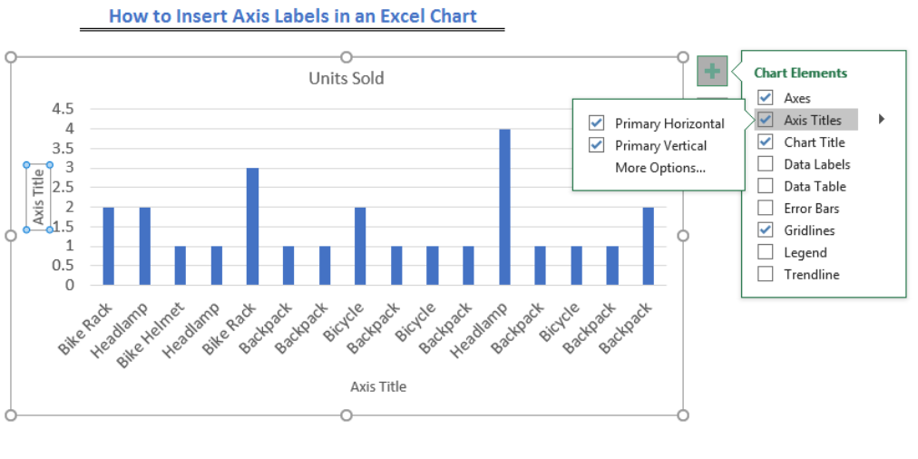
How to Insert Axis Labels In An Excel Chart | Excelchat
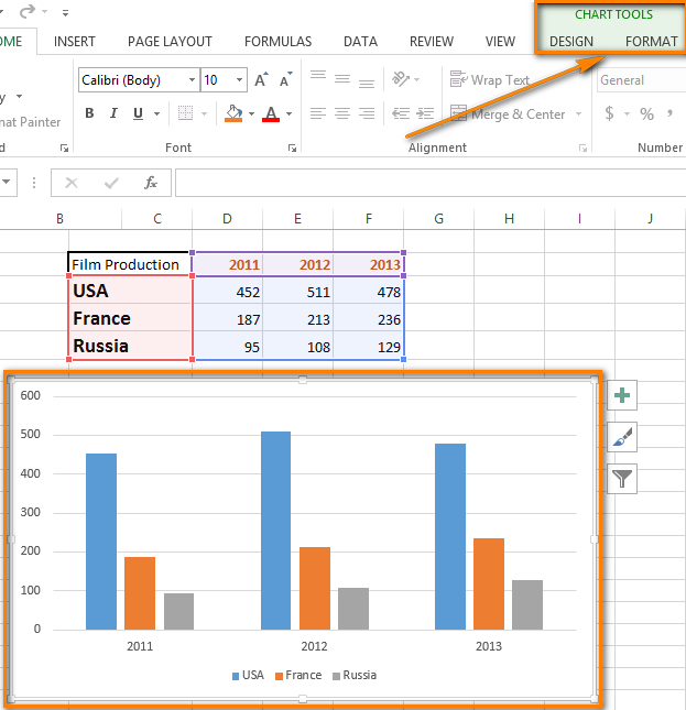
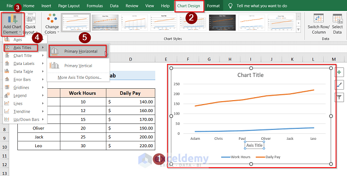
How to Add Axis Titles in a Microsoft Excel Chart - How-To Geek Select your chart and then head to the Chart Design tab that displays. Click the Add Chart Element drop-down arrow and move your cursor to Axis Titles. In the pop-out menu, select "Primary Horizontal," "Primary Vertical," or both. If you're using Excel on Windows, you can also use the Chart Elements icon on the right of the chart.
How to Add Axis Labels in Microsoft Excel - Appuals.com
Excel 2013 - Chart loses axis labels when grouping (hiden) values I can reproduce the behavior with Excel 2013. The only workarounds I've found: - Add the axis label names (Sunday, Monday) manually instead of referring the hidden cells. - Write the label names into a column that is not hidden. When you use Excel 2010 to assign the axis labels, it works also in Excel 2013... till you save the file in Excel 2013.
How to Add Axis Labels in Microsoft Excel - Appuals.com
How to Add Axis Labels in Microsoft Excel - Appuals.com Click anywhere on the chart you want to add axis labels to. Click on the Chart Elements button (represented by a green + sign) next to the upper-right corner of the selected chart. Enable Axis Titles by checking the checkbox located directly beside the Axis Titles option.
Changing Axis Labels in PowerPoint 2013 for Windows
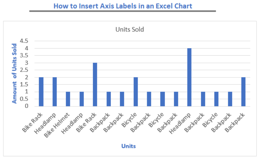
How to Insert Axis Labels In An Excel Chart | Excelchat In Excel 2016 and 2013, we have an easier way to add axis labels to our chart. We will click on the Chart to see the plus sign symbol at the corner of the chart Figure 9 - Add label to the axis We will click on the plus sign to view its hidden menu Here, we will check the box next to Axis title Figure 10 - How to label axis on Excel
Individually Formatted Category Axis Labels - Peltier Tech
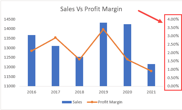
Add or remove a secondary axis in a chart in Excel A secondary axis can also be used as part of a combination chart when you have mixed types of data (for example, price and volume) in the same chart. In this chart, the primary vertical axis on the left is used for sales volumes, whereas the secondary vertical axis on the right side is for price figures. Do any of the following: Add a secondary ...
How to add titles to Excel charts in a minute
How to Create a Pareto Chart in Excel - Automate Excel Step #2: Add data labels. Start with adding data labels to the chart. Right-click on any of the columns and select "Add Data Labels." Customize the color, font, and size of the labels to help them stand out (Home > Font). Step #3: Add the axis titles. As icing on the cake, axis titles provide additional context to what the chart is all about.

How to label x and y axis in Microsoft excel 2016
Individually Formatted Category Axis Labels - Peltier Tech Format the category axis (horizontal axis) so it has no labels. Add data labels to the the dummy series. Use the Below position and Category Names option. Format the dummy series so it has no marker and no line. To format an individual label, you need to single click once to select the set of labels, then single click again to select the ...
Change the display of chart axes
Two-Level Axis Labels (Microsoft Excel) - tips Put your second major group title into cell E1. In cells B2:G2 place your column labels. Select cells B1:D1 and click the Merge and Center tool. (In Excel 2007 the Merge and Center tool is in the Alignment group of the Home tab on the ribbon.) The first major group title should now be centered over the first group of column labels.
How to change chart axis labels' font color and size in Excel?
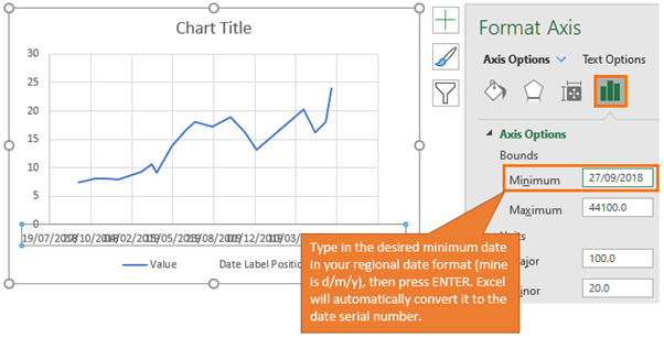
Label Specific Excel Chart Axis Dates • My Online Training Hub
How to Add a Secondary Axis in Excel Charts (Easy Guide ...

How to Insert Axis Labels In An Excel Chart | Excelchat
How to Add X and Y Axis Labels in Excel (2 Easy Methods ...
Excel: Labeling Sparklines - Excel Articles
How to Insert Axis Labels In An Excel Chart | Excelchat
How to Add X and Y Axis Labels in Excel (2 Easy Methods ...

How to add axis label to chart in Excel?

How To Add Axis Labels In Excel - BSUPERIOR

How to Add an Axis Title to an Excel Chart | Techwalla
r - Multi-row x-axis labels in ggplot line chart - Stack Overflow
How to Add Axis Labels in Excel 2013
Change the display of chart axes
How to Add Axis Titles in Excel (2 Quick Methods) - ExcelDemy
Add or remove titles in a chart
How to Customize Your Excel Pivot Chart and Axis Titles - dummies

charts - Can't edit horizontal (catgegory) axis labels in ...
Adding chart title and axis-titles - YouTube

Excel Custom Chart Labels • My Online Training Hub
How to add axis label to chart in Excel?
How to add titles to Excel charts in a minute
Change axis labels in a chart
How to add axis label to chart in Excel?
Change the display of chart axes
Charts | Empirical Reasoning Center Barnard College
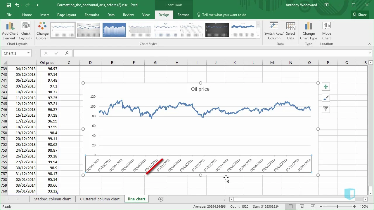
Formatting the Horizontal Axis | Online Excel - KPMG Tax - Digital Now Course Training
Text Labels on a Vertical Column Chart in Excel - Peltier Tech
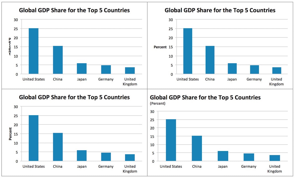
Where to Position the Y-Axis Label - PolicyViz
Post a Comment for "45 how to add axis labels in excel 2013"