38 how to add data labels to a pie chart in excel
Add or remove data labels in a chart - support.microsoft.com For example, in the pie chart below, without the data labels it would be difficult to tell that coffee was 38% of total sales. Depending on what you want to highlight on a chart, you can add labels to one series, all the series (the whole chart), or one data point. Add data labels. You can add data labels to show the data point values from the ... How to Make a PIE Chart in Excel (Easy Step-by-Step Guide) Here are the steps to format the data label from the Design tab: Select the chart. This will make the Design tab available in the ribbon. In the Design tab, click on the Add Chart Element (it's in the Chart Layouts group). Hover the cursor on the Data Labels option. Select any formatting option from the list.
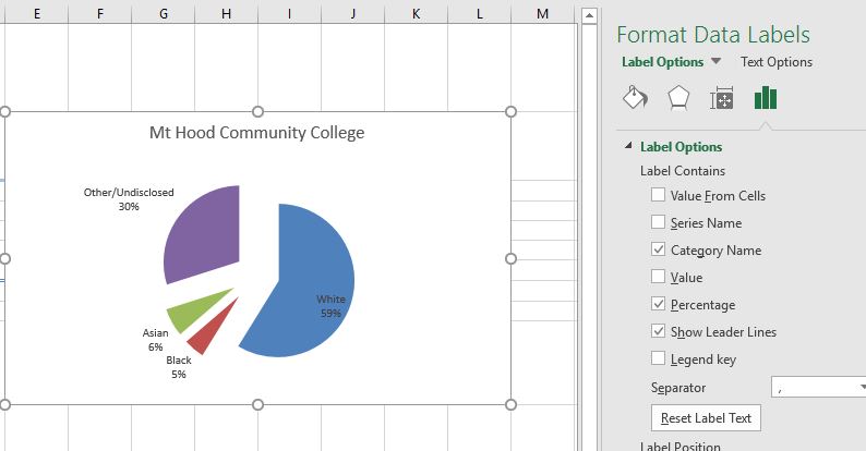
Change the format of data labels in a chart To get there, after adding your data labels, select the data label to format, and then click Chart Elements > Data Labels > More Options. To go to the appropriate area, click one of the four icons ( Fill & Line, Effects, Size & Properties ( Layout & Properties in Outlook or Word), or Label Options) shown here.

How to add data labels to a pie chart in excel
Add data labels and callouts to charts in Excel 365 - EasyTweaks.com The steps that I will share in this guide apply to Excel 2021 / 2019 / 2016. Step #1: After generating the chart in Excel, right-click anywhere within the chart and select Add labels . Note that you can also select the very handy option of Adding data Callouts. Pie Chart Examples | Types of Pie Charts in Excel with Examples Now our task is to add the Data series to the PIE chart divisions. Click on the PIE chart so that the chart will get a highlight, as shown below. Right-click and choose the “Add Data Labels “option for additional drop-down options. Create A Pie Chart In Excel With and Easy Step-By-Step Guide However, it is recommended that you add the actual values from the dataset to every slice of the pie chart. They are known as data labels. If you want to add the data labels then follow these steps: Step 1: Right-click on any of the slices. Step 2: Click on "Add data labels". This will add values to every slice in the pie chart in Excel.
How to add data labels to a pie chart in excel. Create a Pie Chart in Excel (In Easy Steps) - Excel Easy Create the pie chart (repeat steps 2-3). 7. Click the legend at the bottom and press Delete. 8. Select the pie chart. 9. Click the + button on the right side of the chart and click the check box next to Data Labels. 10. Click the paintbrush icon on the right side of the chart and change the color scheme of the pie chart. How to insert data labels to a Pie chart in Excel 2013 - YouTube 98.4K subscribers This video will show you the simple steps to insert Data Labels in a pie chart in Microsoft® Excel 2013. Content in this video is provided on an "as is" basis with no express or... Possible to add second data label to pie chart? - excelforum.com Re: Possible to add second data label to pie chart? Create the composite label in a worksheet column by concatenating the data in other cells and the nextline character, CHR (10). Now, use this composite label column as the source for Rob Bovey's add-in. -- Regards, Tushar Mehta Excel, PowerPoint, and VBA add-ins, tutorials How to Create Bar of Pie Chart in Excel? Step-by-Step Excel lets us add our own customizations to the Bar of Pie chart. For example, it lets us specify how we want the portions to get split between the pie and the stacked bar. It also lets us specify whether we want to display data labels, what data labels we want to be displayed as well as what formatting and styling we want to apply to the labels.
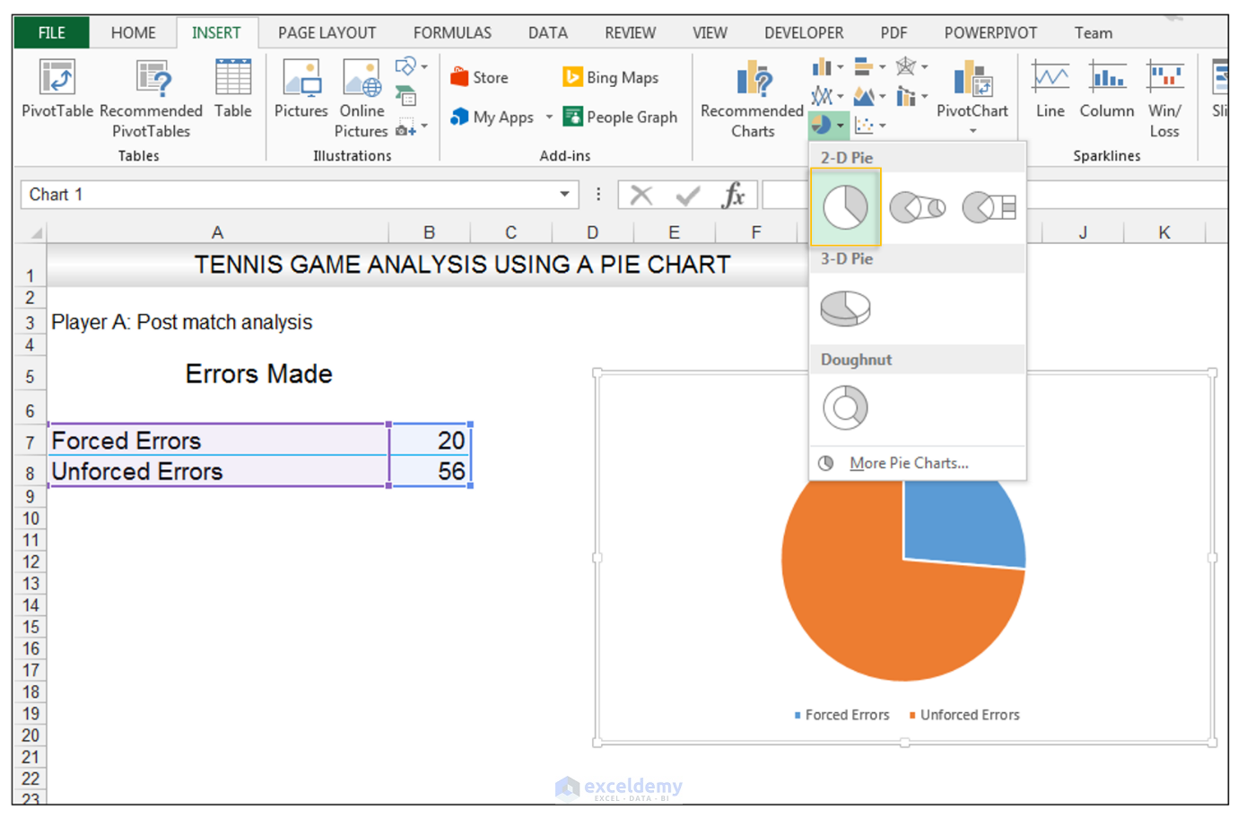
Adding data labels to a pie chart - Excel General - OzGrid Free Excel ... Re: Adding data labels to a pie chart Yes it doesn't appear via intelli-sense unless you use a Series object. Code Dim objSeries As Series Set objSeries = ActiveChart.SeriesCollection (1) objSeries.HasDataLabels [h4] Cheers Andy [/h4] norie Super Moderator Reactions Received 8 Points 53,548 Posts 10,650 Feb 25th 2005 #9 Add a pie chart - support.microsoft.com To switch to one of these pie charts, click the chart, and then on the Chart Tools Design tab, click Change Chart Type. When the Change Chart Type gallery opens, pick the one you want. See Also. Select data for a chart in Excel. Create a chart in Excel. Add a chart to your document in Word. Add a chart to your PowerPoint presentation Legends in Chart | How To Add and Remove Legends In Excel Chart… A Legend is a representation of legend keys or entries on the plotted area of a chart or graph, which are linked to the data table of the chart or graph. By default, it may show on the bottom or right side of the chart. The data in a chart is organized with a combination of Series and Categories. Select the chart and choose filter then you will ... How to Make a Pie Chart in Excel & Add Rich Data Labels to The Chart! 08.09.2022 · A pie chart is used to showcase parts of a whole or the proportions of a whole. There should be about five pieces in a pie chart if there are too many slices, then it’s best to use another type of chart or a pie of pie chart in order to showcase the data better. In this article, we are going to see a detailed description of how to make a pie chart in excel.
How to Add Data Labels to an Excel 2010 Chart - dummies Select where you want the data label to be placed. Data labels added to a chart with a placement of Outside End. On the Chart Tools Layout tab, click Data Labels→More Data Label Options. The Format Data Labels dialog box appears. How to Create a Pie Chart in Excel | Smartsheet Enter data into Excel with the desired numerical values at the end of the list. Create a Pie of Pie chart. Double-click the primary chart to open the Format Data Series window. Click Options and adjust the value for Second plot contains the last to match the number of categories you want in the "other" category. How to Make a Pie Chart in Excel: 10 Steps (with Pictures) - wikiHow 1. Open Microsoft Excel. It resembles a white "E" on a green background. If you would rather make a chart from data you already have, double-click the Excel document that contains the data to open it and proceed to the next section. 2. Click Blank workbook (PC) or Excel Workbook (Mac). Add Data Points to Existing Chart – Excel & Google Sheets Adding Single Data point. Add Single Data Point you would like to ad; Right click on Line; Click Select Data . 4. Select Add . 5. Update Series Name with New Series Header. 6. Update Values . Final Graph with Single Data point . Add a Single Data Point in Graph in Google Sheets
How to Make a Pie Chart in Excel
How to☝️Create a Pie of Pie Chart in Excel - SpreadsheetDaddy Let's take a look at how to add data points to your chart. Right-click on the chart. Select the Add Data Labels option. If you want the labels to be more visually appealing, you can change their color as well. Select the labels. Go to the Home menu. Navigate to the Font section and click on the Font Color option.

Add or remove data labels in a chart
How to Customize Your Excel Pivot Chart Data Labels - dummies To add data labels, just select the command that corresponds to the location you want. To remove the labels, select the None command. If you want to specify what Excel should use for the data label, choose the More Data Labels Options command from the Data Labels menu. Excel displays the Format Data Labels pane.

Adding Data Labels to Your Chart (Microsoft Excel)
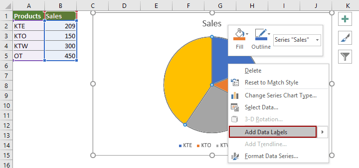
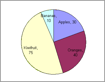
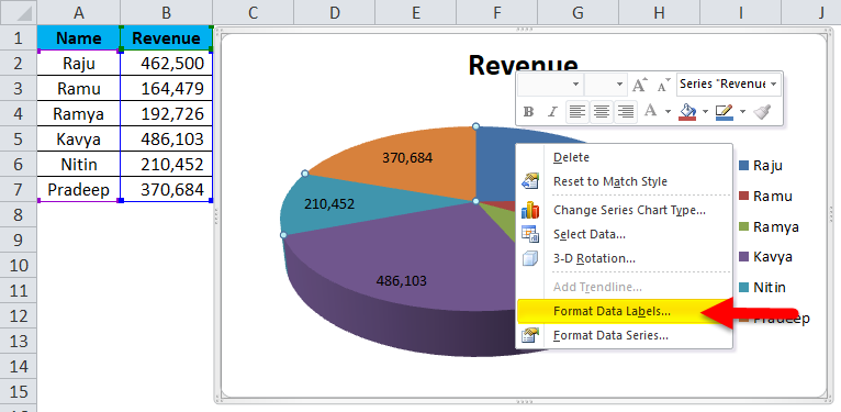
Microsoft Excel Tutorials: Add Data Labels to a Pie Chart - Home and Learn To add the numbers from our E column (the viewing figures), left click on the pie chart itself to select it: The chart is selected when you can see all those blue circles surrounding it. Now right click the chart. You should get the following menu: From the menu, select Add Data Labels. New data labels will then appear on your chart:
How to show percentage in pie chart in Excel?
Pie Chart in Excel | How to Create Pie Chart - EDUCBA Step 1: Do not select the data; rather, place a cursor outside the data and insert one PIE CHART. Go to the Insert tab and click on a PIE. Step 2: once you click on a 2-D Pie chart, it will insert the blank chart as shown in the below image. Step 3: Right-click on the chart and choose Select Data. Step 4: once you click on Select Data, it will ...

Inserting Data Label in the Color Legend of a pie chart ...
Pie Chart in Excel - Inserting, Formatting, Filters, Data Labels Click on the Instagram slice of the pie chart to select the instagram. Go to format tab. (optional step) In the Current Selection group, choose data series "hours". This will select all the slices of pie chart. Click on Format Selection Button. As a result, the Format Data Point pane opens.
Pie Chart Rounding in Excel - Peltier Tech
Excel Pie Chart - How to Create & Customize? (Top 5 Types) Step 1: Click on the Pie Chart > click the ' + ' icon > check/tick the " Data Labels " checkbox in the " Chart Element " box > select the " Data Labels " right arrow > select the " More Options… ", as shown below. The " Format Data Labels" pane opens.

information graphics - How to display data labels in ...
How to Create and Format a Pie Chart in Excel - Lifewire To add data labels to a pie chart: Select the plot area of the pie chart. Right-click the chart. Select Add Data Labels . Select Add Data Labels. In this example, the sales for each cookie is added to the slices of the pie chart. Change Colors
Adding data labels to a Pie Chart in VBA - Automate Excel
Create a pie chart from distinct values in one column by grouping data … Select your data (both columns) and create a Pivot Table: On the Insert tab click on the PivotTable | Pivot Table (you can create it on the same worksheet or on a new sheet) On the PivotTable Field List drag Country to Row Labels and Count to Values if Excel doesn't automatically. Now select the pivot table data and create your pie chart as ...
How to Make a Pie Chart in Excel & Add Rich Data Labels to ...
How to Edit Pie Chart in Excel (All Possible Modifications) Just like the chart title, you can also change the position of data labels in a pie chart. Follow the steps below to do this. 👇 Steps: Firstly, click on the chart area. Following, click on the Chart Elements icon. Subsequently, click on the rightward arrow situated on the right side of the Data Labels option.

How to Create a Pie Chart in Excel - Displayr
Inserting Data Label in the Color Legend of a pie chart Hi, I am trying to insert data labels (percentages) as part of the side colored legend, rather than on the pie chart itself, as displayed on the image ... but you can use a trick: see Add Percent Values in Pie Chart Legend (Excel 2010) 0 Likes . Reply. Share. Share to LinkedIn; Share to Facebook; Share to Twitter; Share to Reddit;

Automatically Group Smaller Slices in Pie Charts to one big Slice
Office: Display Data Labels in a Pie Chart - Tech-Recipes: A Cookbook ... 2. If you have not inserted a chart yet, go to the Insert tab on the ribbon, and click the Chart option. 3. In the Chart window, choose the Pie chart option from the list on the left. Next, choose the type of pie chart you want on the right side. 4. Once the chart is inserted into the document, you will notice that there are no data labels.
Help Online - Quick Help - FAQ-1017 How to recover the ...
How to display leader lines in pie chart in Excel? - ExtendOffice To display leader lines in pie chart, you just need to check an option then drag the labels out. 1. Click at the chart, and right click to select Format Data Labels from context menu. 2. In the popping Format Data Labels dialog/pane, check Show Leader Lines in the Label Options section. See screenshot: 3. Close the dialog, now you can see some ...
4.1.3 Choosing a Chart Type: Pie Chart – Excel For Decision ...
Adding Data Labels to Your Chart (Microsoft Excel) - ExcelTips (ribbon) To add data labels in Excel 2013 or later versions, follow these steps: Activate the chart by clicking on it, if necessary. Make sure the Design tab of the ribbon is displayed. (This will appear when the chart is selected.) Click the Add Chart Element drop-down list. Select the Data Labels tool.

vba - Excel Prevent overlapping of data labels in pie chart ...
How to Add and Remove Chart Elements in Excel Select the data, go to insert menu --> Charts --> Line Chart. 1: Add Data Label Element to The Chart. To add the data labels to the chart, click on the plus sign and click on the data labels. This will ad the data labels on the top of each point. If you want to show data labels on the left, right, center, below, etc. click on the arrow sign. It ...
5 New Charts to Visually Display Data in Excel 2019 - dummies
Multiple data labels (in separate locations on chart) Running Excel 2010 2D pie chart I currently have a pie chart that has one data label already set. The Pie chart has the name of the category and value as data labels on the outside of the graph. I now need to add the percentage of the section on the INSIDE of the graph, centered within the pie section.

How to show percentage in pie chart in Excel?
How To Make A Pie Chart In Excel: In Just 2 Minutes [2022] When you first create a pie chart, Excel will use the default colors and design.. But if you want to customize your chart to your own liking, you have plenty of options. The easiest way to get an entirely new look is with chart styles.. In the Design portion of the Ribbon, you’ll see a number of different styles displayed in a row. Mouse over them to see a preview:

how to add data labels into Excel graphs — storytelling with data
How to Add Axis Labels in Excel Charts - Step-by-Step (2022) Left-click the Excel chart. 2. Click the plus button in the upper right corner of the chart. 3. Click Axis Titles to put a checkmark in the axis title checkbox. This will display axis titles. 4. Click the added axis title text box to write your axis label. Or you can go to the 'Chart Design' tab, and click the 'Add Chart Element' button ...
Create a Pie Chart in Excel (In Easy Steps)
How to add data labels from different column in an Excel chart? Right click the data series in the chart, and select Add Data Labels > Add Data Labels from the context menu to add data labels. 2. Click any data label to select all data labels, and then click the specified data label to select it only in the chart. 3.

How-to Add Label Leader Lines to an Excel Pie Chart - Excel ...
Create A Pie Chart In Excel With and Easy Step-By-Step Guide However, it is recommended that you add the actual values from the dataset to every slice of the pie chart. They are known as data labels. If you want to add the data labels then follow these steps: Step 1: Right-click on any of the slices. Step 2: Click on "Add data labels". This will add values to every slice in the pie chart in Excel.

How to show percentages on three different charts in Excel ...
Pie Chart Examples | Types of Pie Charts in Excel with Examples Now our task is to add the Data series to the PIE chart divisions. Click on the PIE chart so that the chart will get a highlight, as shown below. Right-click and choose the “Add Data Labels “option for additional drop-down options.
Excel Doughnut chart with leader lines – teylyn
Add data labels and callouts to charts in Excel 365 - EasyTweaks.com The steps that I will share in this guide apply to Excel 2021 / 2019 / 2016. Step #1: After generating the chart in Excel, right-click anywhere within the chart and select Add labels . Note that you can also select the very handy option of Adding data Callouts.

Create Outstanding Pie Charts in Excel | Pryor Learning
When to use Pie Charts in Dashboards - Best Practices | Excel ...
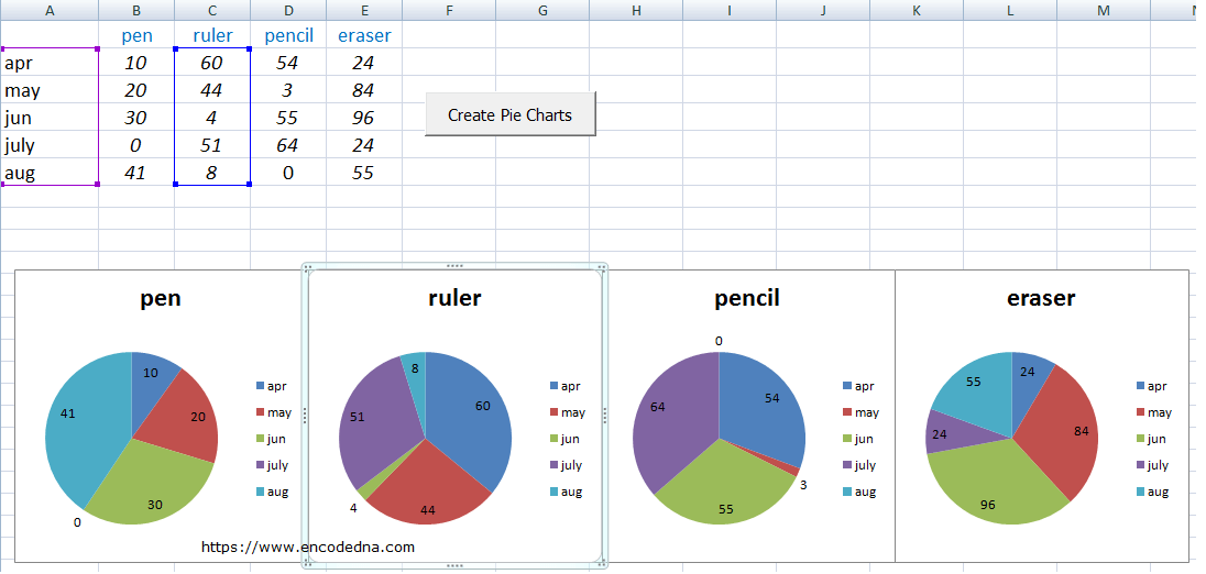
Create Multiple Pie Charts in Excel using Worksheet Data and VBA
Office: Display Data Labels in a Pie Chart

Creating Graphs in Excel 2013

Excel: How to not display labels in pie chart that are 0 ...

How to Make Pie Chart with Labels both Inside and Outside ...
/Capture-5c8489fbc9e77c0001422f49.JPG)
How to Create and Format a Pie Chart in Excel
Pie Chart in Excel | How to Create Pie Chart | Step-by-Step ...
How to Make a Pie Chart in Excel & Add Rich Data Labels to ...

How to Make a Pie Chart in Excel - All Things How

How to Make a PIE Chart in Excel (Easy Step-by-Step Guide)
How to ☝️Make a Pie Chart in Excel (Free Template ...

Presenting Data with Charts
How to Create a Pie Chart in Excel using Worksheet Data

How to fix wrapped data labels in a pie chart | Sage Intelligence

How to Make an Excel Pie Chart
Post a Comment for "38 how to add data labels to a pie chart in excel"