42 excel donut chart labels

How to Create Curved Labels in Excel Doughnut Chart (With Easy Steps) In this article, we will learn to create curved labels in an Excel doughnut chart. Doughnut charts are used to represent a 'part-to-whole' relationship. All the parts together form 100 %. Unfortunately, you can not create curved labels in a doughnut chart. By default, the labels are expressed in a straight line. But we can take the help of ... Curve Text in Doughnut chart - Excel Help Forum Re: Curve Text in Doughnut chart. You can link WordArt to a cell using a formula. Just select the shape, click into the formula bar, type = and then select the cell and press Enter. Please remember to mark your thread 'Solved' when appropriate.

Add / Move Data Labels in Charts - Excel & Google Sheets Add and Move Data Labels in Google Sheets. Double Click Chart. Select Customize under Chart Editor. Select Series. 4. Check Data Labels. 5. Select which Position to move the data labels in comparison to the bars.

Excel donut chart labels

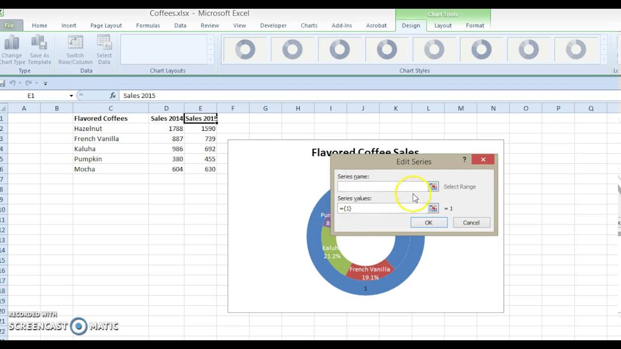
Donut/Doughnut Chart - Multiple Series - Microsoft Tech Community I have created a doughnut chart with multiple series (represented by multiple rings - see charts below). Each ring is divided into 6, the colour of which corresponds to one of three options (yes, maybe and no). I therefore want the colour of the chart to represent this clearly (green, yellow and red... How to Create a Double Doughnut Chart in Excel - Statology Step 3: Add a layer to create a double doughnut chart. Right click on the doughnut chart and click Select Data. In the new window that pops up, click Add to add a new data series. For Series values, type in the range of values fpr Quarter 2 revenue: Click OK. Question: labels in an Excel doughnut chart - Microsoft Tech Community Open your Excel document and click on your chart. In the upper bar you will find the "Diagram Tools". Click on the "Design" tab. In the "Data" group, click the "Select data" button. In the right window you will find the "Horizontal axis label". Click on "Edit". Now enter your desired names or values for the legend.

Excel donut chart labels. How to Make a Doughnut Chart in Excel (2 Suitable Examples) You will see that data labels have been added to your chart.After that, you can select any other format you want for your doughnut chart.. Firstly, select the chart. Secondly, go to Chart Styles.; Thirdly, select Style.; Finally, you can select any chart format from there. How to create doughnut chart in Excel? - ExtendOffice In Excel 2013, click Insert > Insert Pie or Doughnut Chart > Doughnut. See screenshot: 2. Then a doughnut chart is inserted in your worksheet. Now you can right click at all series and select Add Data Labels from the context menu to add the data labels. See screenshots: Now a simple doughnut chart is created. Fix label position in doughnut chart? | MrExcel Message Board Turn off data labels. Insert a Text box in to the middle of the donut, select the edge of the text box and in the formula bar hit = then select the cell that contains the progress figure. You can format this to however you want it, it will update and it won't move. Click to expand... Oh wow! I always thought text-boxes were just text-boxes. How to Create Doughnut Excel Chart? - WallStreetMojo A doughnut chart is a chart in Excel whose visualization function is similar to pie charts. The categories represented in this chart are parts, and together they express the whole data in the chart. We can only use the data in rows or columns in creating a doughnut chart in Excel.

donut chart labels - Microsoft Community Click the chart. On the Format tab, in the Size group, enter the size that you want in the Shape Height and Shape Width box. Tip For our doughnut chart, we set the shape height to 4" and the shape width to 5.5". To change the size of the doughnut hole, do the following: How to Create Doughnut Chart in Excel? - EDUCBA Now we will create a doughnut chart as similar to the previous single doughnut chart. Select the data alone without headers, as shown in the below image. Click on the Insert menu. Go to charts select the PIE chart drop-down menu. From Dropdown, select the doughnut symbol. Then the below chart will appear on the screen with two doughnut rings. Excel Charts - Doughnut Chart - tutorialspoint.com Doughnut charts show the size of items in a data series, proportional to the sum of the items. The doughnut chart is similar to a pie chart, but it can contain more than one data series. Step 1 − Arrange the data in columns or rows on the worksheet. Step 2 − Select the data. Step 3 − On the INSERT tab, in the Charts group, click the Pie ... How to create a creative multi-layer Doughnut Chart in Excel By default, all doughnut chart layers have a borderline. As this border line is only disrupting the look, you should remove it for all borders first. After that, select the outer layer of the second (also second biggest) data point and set the fill to No fill. For the third data point we apply the same technique to the two outer layers, and so on.

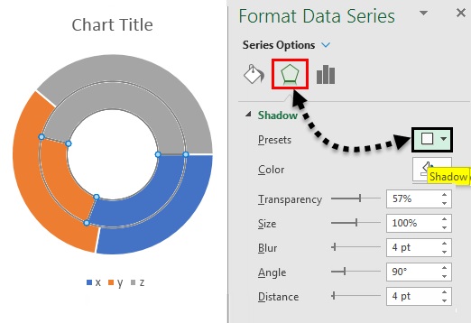
Progress Doughnut Chart with Conditional Formatting in Excel The entire chart will be shaded with the progress complete color, and we can display the progress percentage in the label to show that it is greater than 100%. Step 2 - Insert the Doughnut Chart With the data range set up, we can now insert the doughnut chart from the Insert tab on the Ribbon. The Doughnut Chart is in the Pie Chart drop-down menu. Change the format of data labels in a chart To get there, after adding your data labels, select the data label to format, and then click Chart Elements > Data Labels > More Options. To go to the appropriate area, click one of the four icons ( Fill & Line, Effects, Size & Properties ( Layout & Properties in Outlook or Word), or Label Options) shown here. Half Donut Chart (Infographic Style ) - Beat Excel! Now select range C3:E13 and insert a donut chart. The chart you see will look like the one below: Press Switch Row/Column button from chart tools menu and it will look more like the chart we are making. Chart Tools menu will be activated after you click on the chart. Now click on chart title and delete it. Labels for pie and doughnut charts - Support Center To format labels for pie and doughnut charts: 1. Select your chart or a single slice. Turn the slider on to Show Label. 2. Use the sliders to choose whether to include Name, Value, and Percent. When Show Label and Percent are selected, you will also have the option to select Round labels to 100% . Note: Rounding labels to 100% is done by force ...

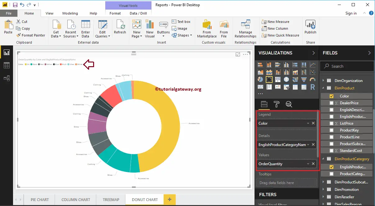
Create a Power BI Donut Chart

How to make doughnut chart with outside end labels? - Simple Excel VBA ... In the doughnut type charts Excel gives You no option to change the position of data label. The only setting is to have them inside the chart.

Doughnut Chart in Excel | How to Create Doughnut Chart in Excel?

How to Make a Doughnut Chart in Excel | EdrawMax Online How to Make a Doughnut Chart in EdrawMax Step 1: Select Chart Type When you open a new drawing page in EdrawMax, go to Insert tab, click Chart or press Ctrl + Alt + R directly to open the Insert Chart window so that you can choose the desired chart type.

Doughnut Chart in Excel | How to Create Doughnut Chart in Excel?

Excel Doughnut chart with leader lines - teylyn Step 1 - doughnut chart with data labels Step 2 -Add the same data series as a pie chart Next, select the data again, categories and values. Copy the data, then click the chart and use the Paste Special command. Specify that the data is a new series and hit OK. You will see the new data series as an outer ring on the doughnut chart.

33 How To Label Pie Chart - Labels Database 2020

Prevent Overlapping Data Labels in Excel Charts - Peltier Tech Here is the chart after running the routine, without allowing any overlap between labels (OverlapTolerance = zero).All labels can be read, but the space between them is greater than needed (you could almost stick another label between any two adjacent labels here), and some labels have moved far from the points they label.

How to create a donut chart - Datawrapper Academy

Present your data in a doughnut chart - support.microsoft.com To add text labels with arrows that point to the doughnut rings, do the following: On the Layout tab, in the Insert group, click Text Box. Click on the chart where you want to place the text box, type the text that you want, and then press ENTER.

Interactive Donut Chart - Beat Excel!

How to add leader lines to doughnut chart in Excel? Select data and click Insert > Other Charts > Doughnut. In Excel 2013, click Insert > Insert Pie or Doughnut Chart > Doughnut. 2. Select your original data again, and copy it by pressing Ctrl + C simultaneously, and then click at the inserted doughnut chart, then go to click Home > Paste > Paste Special. See screenshot: 3.

Pie Chart in Excel | Pie Graph | QI Macros Excel Add-in

Excel Doughnut Chart in 3 minutes - Watch Free Excel Video ... - YouTube Doughnut charts is cirular graph which display data in rings, where each ring represents a data series. In Doughnut Chart percentages are displayed in data l...

How to Create a Donut Chart in Microsoft Excel - Tutorial - YouTube

excel - Positioning labels on a donut-chart - Stack Overflow The option to place the labels outside the chart is not available on the doughnut chart options: like they do on a pie chart: However, you could perform a trick using a pie chart and a white circle to make it look like a doughnut by doing the following: Sub AddCircle () 'Get chart size and position: Dim CH01 As Chart: Set CH01 = ThisWorkbook ...

How-to Add Label Leader Lines to an Excel Pie Chart - Excel Dashboard Templates

Donut, column, and bar chart dashboard - templates.office.com Add this dashboard including donut, column, and bar charts to any slideshow. This is an accessible template. Add this dashboard including donut, column, and bar charts to any slideshow. ... Excel Find inspiration for your next project with thousands of ideas to choose from. Address books. ... Labels. Learning. Letters. Lists. Logs. Maps. Memos ...

Add label to center of C# Excel Doughnut chart - Stack Overflow

Question: labels in an Excel doughnut chart - Microsoft Tech Community Open your Excel document and click on your chart. In the upper bar you will find the "Diagram Tools". Click on the "Design" tab. In the "Data" group, click the "Select data" button. In the right window you will find the "Horizontal axis label". Click on "Edit". Now enter your desired names or values for the legend.

How to Create a Double Doughnut Chart in Excel - Statology

How to Create a Double Doughnut Chart in Excel - Statology Step 3: Add a layer to create a double doughnut chart. Right click on the doughnut chart and click Select Data. In the new window that pops up, click Add to add a new data series. For Series values, type in the range of values fpr Quarter 2 revenue: Click OK.